Work around needed for lack of drop down menus in Numbers

[gmacdowellpsyd]

I need to be able to transfer information from one page of the worksheet to a summary page in the same worksheet, so that I can print out the summary for my clients. On the first page will be multiple checkboxes so that I can quickly record which product the client desires for each purpose. I don't want to give them this entire form, so I need to transfer to the summary form just the information in the column adjacent to whatever checkboxes are checked during the consultation. I presume there is some sort of formula with an IF-THEN kind of statement, but I am not well versed at these things. Anyone know how to transfer the text of a box to another location ONLY when the adjacent checkbox is checked? Thanks in advance.

 

[twerppoet]

You're on the right track with the IF Statement. I did a quick couple sheets that may be close to what you want to do. The first attachment is the origin sheet with the checkmark and value cells. The second attachment is the summary sheet with the formula.

The fist part of the IF statement tests if the checkmark cell is true (checked). The second says what to do if it is true (display this cell), and the third says what to do if the test was not true (display N/A).

If you are going to try and add a sum at the bottom, better to set the cell to zero when not true.

If you can't figure out how to create the formula, let me know. I'll try to give a step by step, but I'm going to be busy this weekend, so I don't know when I'll get to it.

 

[gmacdowellpsyd]

I appreciate your efforts. I tried to duplicate the formula but did not know how to get the little triangles into it. Numbers reported a syntax error. The info to be transferred is text, not numeric. Also, If possible, I would like the "false" to reflect no entry in the column.

There will be upwards of 7 different boxes to be possibly checked for any one row in sheet 1. These represent 7 different products. Only one will be selected during the consultation. In a perfect world, that one product would show up on the summary sheet on its own row in the same column. I suspect that is too much to expect.

Also, as I work on the sheet, the checkbox on sheet 1 disappears and a 1 shows up in the cell when I try to uncheck the box. Inasmuch as the keyboard doesn't always show up on the first tap, I am in a quandary as to what is happening overall.

Thanks for your help in advance.

 

[twerppoet]

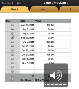
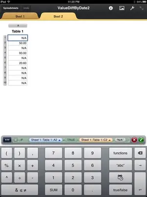
The triangles are just something Numbers puts there when you are referencing another table and/or sheet. I'm not sure exactly what, but it is nothing you can enter directly.

You get the Sheet:Table:Cell reference by selecting the part of the formula you want (tap on it and it highlights), then navigating to that Sheet, Table, and cell; and tapping on it.

This formula should work for either text or numeric values. I just happened to have a spread sheet set up that was easy to play with, and it had a column of numbers, not text.

To check a box, double tap on the cell to get the cell editor. You can switch between true and false either by tapping on the cell again, or by tapping on the text entry field in the editor. Tapping on the check mark key changes the format of the cell back and forth between numeric and check box, which is why you keep getting a '1'.

What you want to do is getting complicated to describe. After your third post you'll be able to post links and add attachments to your posts. I recommend you set up the basic tables the way you want (sans sensitive data), label them, describe what you want to happen in each cell, row, column, and post it here.

I'll give it a shot, but no promises. Some of what you are describing (only the checked item showing up on the Summary), is going be challenging, which is why I'm interested. It will be fun trying to figure out what functions to use, and how to string them together.

In the mean time I'll do a step by step on how to create this formula (even though it probably isn't exactly what you want). That will give you a good idea of how to create any formula you see or come up with yourself.

The Undo button at the top left of the screen can be a big help when you accidentally tap the wrong cell or key.

1) Double tap on the cell you want to create the formula (A1 in this case), then tap on the = sign to enter formula entry mode in the cell editor.

2) Tap the functions key, the Categories tab, Logical and Information, then IF. You'll see the IF expression with placeholders: if-expression, if-true, if-false.

3) The first place holder, if-expression, is already highlighted. If not tap it once to do so.

4) Navigate to the Sheet, Table, and cell to be tested and tap that cell. In this case it was Sheet 1::Table 1::A2.

5) On the operations keypad (left block of keys) tap the bottom key to get more operations, then tap the = key.

6) Tap the functions key, Categories, Logical and Information, then TRUE. This completes the first part of the IF function. It tests if Cell A2, Table 1, Sheet 1 is true (the box is checked)

The next part of the statement (if-true) is what happens if the box is checked (tests true).

7) Tap the if-true placeholder so that it is highlighted. Now go to the cell you want to display on the summary page, in this case Sheet 1::Table 1::C2, and tap it.

The last part says what to do if the check box is not checked.

8) Tap the if-flase placeholder to select it. Now tap the "abc" key and enter the text you want to appear when the check box is not selected. This could be anything, including not text at all. IN this case I chose the old standby N/A. You could type nothing and hit Done to get a blank cell.

9) Tap the green checkmark to finish and error check the formula.